基础操作

查看数据类型:

1
> class(spam)
[1] "data.frame"

安装包:

1
install.packages("ElemStatLearn")

使用包:

1
library(ElemStatLearn)

数据结构

1. Vectors

1
2
3
4
5
6
7
8
9
10
11
12
13
14
15
16
17
18
19
20
21
22
23
24
25
26
27
28
# 创建向量
a <-c(1, 2, 3, 4, 5, 6)
b <-c("one", "two", "three")
c <-c(TRUE, FALSE, TRUE, TRUE, FALSE)

> 5:1
[1] 5 4 3 2 1

> 2*(1:5)
[1] 2 4 6 8 10

> rep(1,9)
[1] 1 1 1 1 1 1 1 1 1

> rep(c(1,0,4), each=3)
[1] 1 1 1 0 0 0 4 4 4

> seq(1,3, by=0.2)
> seq(from=1, to=3, by=0.2)
[1] 1.0 1.2 1.4 1.6 1.8 2.0 2.2 2.4 2.6 2.8 3.0

> seq(3,1, by=-0.2)
[1] 3.0 2.8 2.6 2.4 2.2 2.0 1.8 1.6 1.4 1.2 1.0
> seq(3,1, by=0.2)
Error in seq.default(3, 1, by = 0.2) : wrong sign in 'by' argument

> seq(3,1.1)
[1] 3 2
1
2
3
4
5
6
7
# 向量索引
a[2] # 第二个元素
# [1] 2
a[-2] # 删除第二个元素,a 还是原来的 a
# [1] 1 3 4 5 6
a[c(2:4)] # 取出第二到第四个元素
# [1] 2 3 4

2. 矩阵

二维数组

1
2
# 创建矩阵
mymat <- matrix(c(1:10), nrow=2, ncol=5, byrow=TRUE)

得到:

1
2
3
     [,1] [,2] [,3] [,4] [,5]
[1,] 1 2 3 4 5
[2,] 6 7 8 9 10
1
2
3
4
#矩阵索引
mymat[2,] # 取第二行
mymat[,2] # 取第二列
mymat[1,5] # 第一行第五列的元素
1
2
nrow(mymat)  # 获取行数
ncol(mymat) # 获取列数

3. 数组

维度可以大于 2

1
2
# 创建数组
myarr <- array(c(1:12),dim=c(2,3,2))

得到:

1
2
3
4
5
6
7
8
9
10
11
, , 1

[,1] [,2] [,3]
[1,] 1 3 5
[2,] 2 4 6

, , 2

[,1] [,2] [,3]
[1,] 7 9 11
[2,] 8 10 12
1
2
3
4
dim(myarr) # 取矩阵或数组的维度
# [1] 2 3 2
myarr[1,2,1] # 取第一个矩阵的第一行第二列
# [1] 3

4. Data Frame

类似矩阵,每一列可以有不同的模式

1
2
3
4
# 创建数据框
kids <- c("Wang", "Li")
age <- c("18", "16")
df <- data.frame(kids, age)

得到:

1
2
3
  kids age
1 Wang 18
2 Li 16
1
2
3
4
5
6
7
8
9
10
11
12
13
14
15
16
17
18
19
20
21
22
23
24
25
#数据框索引
df[1,] # 第一行
df[,2] # 第二列
df[1:2,1:2] # 前两行,前两列
df$age # 根据列名称

> df$age
[1] 18 16
Levels: 16 18

#数据框常用函数
str(df) # 数据框的结构

> str(df)
'data.frame': 2 obs. of 2 variables:
$ kids: Factor w/ 2 levels "Li","Wang": 2 1
$ age : Factor w/ 2 levels "16","18": 2 1

rownames(df) # 行名称
colnames(df) # 列名称

> rownames(df)
[1] "1" "2"
> colnames(df)
[1] "kids" "age"

更换列名:

1
colnames(m) <- c("Date", "Bill", "Dollar", "Gold")

最小值:

1
min(m$Gold, na.rm=T)

其中 na.rm=T 是为了防止 na 值影响结果,会移除 na 数据

合并

根据某一共同列合并:

1
2
3
4
5
6
7
8
9
10
11
12
13
14
15
16
17
18
19
20
21
# student

SID Course Score
1 11 Math 90
2 11 English 80
3 12 Math 80
4 12 Chinese 95
5 13 Math 96


result <- merge(student,score,by.x="ID",by.y="SID")


# result

ID Name Gender Birthdate Age Course Score
1 11 Devin M 1984-12-29 31 Math 90
2 11 Devin M 1984-12-29 31 English 80
3 12 Edward M 1983-05-06 32 Math 80
4 12 Edward M 1983-05-06 32 Chinese 95
5 13 Wenli F 1986-08-08 29 Math 96

合并多个:

1
m <- Reduce(function(x,y)merge(x, y, by="DATE", all=TRUE), list(data1, data2, data3))

cbind 函数/横向追加

1
2
3
4
5
6
7
8
ID<-c(1,2,3,4)
name<-c("A","B","C","D")
score<-c(60,70,80,90)
sex<-c("M","F","M","M")
student1<-data.frame(ID,name)
student2<-data.frame(score,sex)
total_student2<-cbind(student1,student2)
total_student2

rbind 函数/纵向追加

1
2
3
4
5
6
7
8
ID<-c(1,2,3,4)
name<-c("A","B","C","D")
student1<-data.frame(ID,name)
ID<-c(5,6,7,8)
name<-c("E","F","G","H")
student2<-data.frame(ID,name)
total_student3<-rbind(student1,student2)
total_student3

类型转换

1
2
3
for (i in 1:ncol(df)) {
df[,i] <- as.integer(df[,i]) #将每列类型变为integer型
}

数据清洗

NA 值处理

去除所有含NA的行

1
2
data
data<-na.omit(data)

排序

单变量序列的排序常用到 ranksortorder 函数。

1
2
3
4
5
6
7
> a <- c(3, 1, 5)
> rank(a)
[1] 2 1 3
> sort(a)
[1] 1 3 5
> order(a)
[1] 2 1 3
  • rank 用来计算序列中每个元素的秩,这里的“秩”可以理解为该元素在序列中由小到大排列的次序
  • sort 函数给出的是排序后的结果
  • order 函数给出的是排序后的序列中各元素在原始序列中的位置,序列 [3, 1, 5] 按升序规则排序后的结果是 [1, 3, 5] ,其中 [1, 3, 5] 在原始序列中的位置是 [2, 1, 3]

最大最小值

1
2
3
4
5
6
7
8
9
10
11
12
13
14
15
16
17
18
19
# 新建数组  
a=c(1,3,4,5,3,2,5,6,3,2,5,6,7,5,8)

# 取数组a中最大值的下标
which.max(a)

# 取数组a中最小值的下标
which.min(a)

# 取数组a中大于3值的下标
which(a>3)

# 取数组a中等于3值的下标
which(a==3)

# 10到1的数组元素中在a中的元素的下标
> b <- which(10:1 %in% a)
> b
[1] 3 4 5 6 7 8 9 10

筛选

标准化

中心化:数据 - 均值
标准化:(数据 - 均值)/ 标准差

数据中心化: scale(data,center=T,scale=F)
数据标准化: scale(data,center=T,scale=T) 或默认参数 scale(data)

scale 方法中的两个参数 center 和 scale 的解释:

  1. center 和 scale 默认为真,即 T 或者 TRUE
  2. center 为真表示数据中心化
  3. scale 为真表示数据标准化

实践

读取 CSV

1
2
3
4
5
6
7
8
9
10
read.table(file, header = FALSE, sep = "", quote = "\"'",
dec = ".", numerals = c("allow.loss", "warn.loss", "no.loss"),
row.names, col.names, as.is = !stringsAsFactors,
na.strings = "NA", colClasses = NA, nrows = -1,
skip = 0, check.names = TRUE, fill = !blank.lines.skip,
strip.white = FALSE, blank.lines.skip = TRUE,
comment.char = "#",
allowEscapes = FALSE, flush = FALSE,
stringsAsFactors = default.stringsAsFactors(),
fileEncoding = "", encoding = "unknown", text, skipNul = FALSE)

1
dataset <- read.table("C:\\Datasets\\haberman.csv", header=FALSE, sep=",")
  • 如果第一行数据包含列的名字,则第二个参数应该为:header = TRUE
  • 分割符:
    • 空格: sep = " "
    • tabs: sep = "\t"
    • 默认是 “white space” (one or more spaces, tabs, etc.)

如果分割符号为逗号,那么也可以用 read.csv,并且不用写 seq 参数:

1
dataset <- read.csv("C:\\Datasets\\haberman.csv", header=FALSE)

机器学习算法

KNN

引入 class 包:

1
library(class)

knn() 函数的语法和参数如下:

1
knn(train, test, cl, k = 1, l = 0, prob = FALSE, use.all = TRUE)
  • train:指定训练样本集
  • test :指定测试样本集
  • cl :指定训练样本集中的分类变量
  • k :指定最邻近的k个已知分类样本点,默认为1
  • l :指定待判样本点属于某类的最少已知分类样本数,默认为0
  • prob:设为TRUE时,可以得到待判样本点属于某类的概率,默认为FALSE
  • use.all:控制节点的处理办法,即如果有多个第K近的点与待判样本点的距离相等,默认情况下将这些点都纳入判别样本点,当该参数设为FALSE时,则随机挑选一个样本点作为第K近的判别点
1
2
3
4
5
6
7
8
9
10
11
12
13
> # z-score数据标准化
> iris_scale <- scale(iris[-5])
> train <- iris_scale[c(1:25,50:75,100:125),] #训练集
> test <- iris_scale[c(26:49,76:99,126:150),] #测试集
> train_lab <- iris[c(1:25,50:75,100:125),5]
> test_lab <- iris[c(26:49,76:99,126:150),5]
> pre <- knn(train=train,test=test,cl=train_lab,k=round(sqrt(dim(train)[1])),prob = F)
> table(pre,test_lab)
test_lab
pre setosa versicolor virginica
setosa 24 0 0
versicolor 0 24 3
virginica 0 0 22

实例:

1
2
3
4
5
6
7
8
9
10
11
12
13
14
15
16
17
18
19
20
21
22
23
24
25
26
27
28
29
30
31
32
33
34
35
36
37
38
39
40
41
library(ElemStatLearn)

####################################
## Part 1. Load and Explore Data #
####################################

data(spam)
colnames(spam) <- c(paste("X", 1:57, sep = ""), "spam")
spam$spam <- factor(spam$spam, levels = c("spam", "email"), labels = c("spam", "email"))


#######################
# Normalize Variables #
#######################

spam_n <- as.data.frame(scale(spam[1:57]))


################################################
## Part 2. Creating training and test datasets #
################################################

index <- sample(1:4601, 3000)

spam_train <- spam_n[index, ]
spam_test <- spam_n[-index, ]
spam_train_label <- spam[index, 58]
spam_tset_label <- spam[-index, 58]


########################################
## Part 3. Train the model on the data #
########################################


library(class)

spam_test_pred <- knn(train = spam_train, test = spam_test, cl = spam_train_label, k = 3)
result <- data.frame(spam_tset_label, spam_test_pred)

mean(spam_test_pred == spam_tset_label)

Naive Bayes

实例:

1
2
3
4
5
6
7
8
9
10
11
12
13
14
15
16
17
18
19
20
21
22
23
24
25
26
27
28
29
30
31
32
33
34
35
36
37
38
39
40
41
42
43
44
45
46
47
48
49
50
51
52
53
54
55
56
57
58
59
60
61
62
63
64
65
66
67
68
69
70
71
72
73
74
75
76
77
78
79
80
81
82
83
84
85
86
87
88
89
90
91
92
93
94
95
96
97
98
99
100
101
102
103
104
105
106
107
108
109
110
111
112
113
114
115
116
117
118
119
120
121
122
123
124
125
126
127
128
129
130
131
132
133
134
135
136
137
138
139
140
141
142
143
144
145
146
147
148
149
150
151
152
153
154
155
156
157
158
159
160
161
162
163
164
165
166
167
168
169

###########################################
# Classification with Naive Bayes #
###########################################

setwd("D:/data/ML2019/")
library(data.table) # read text data
library(wordcloud) # make word cloud
library(RColorBrewer) # make word cloud
library(tm) # construct text vector
library(magrittr) # enable pipeline operator
library(e1071) # naive bayes
library(caret) # split data into training and test sets


####################################
## Part 1. Load and Explore Data #
####################################


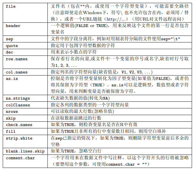
sms_raw <- fread("SMSSpamCollection", header = FALSE, encoding = "Latin-1",sep = "\t", quote="")

colnames(sms_raw)<-c("type", "text")

sms_raw$type <- factor(sms_raw$type)
table(sms_raw[, type])

# ham spam # 4827 747

table(sms_raw[, type]) %>% prop.table()

# ham spam # 0.8659849 0.1340151

##########################
# Word Cloud 词云 #
##########################


pal <- brewer.pal(7, "Dark2")
sms_raw[type == "spam", text] %>%
wordcloud(min.freq = 20,
random.order = FALSE, colors = pal
)
sms_raw[type == "ham", text] %>%
wordcloud(min.freq = 70,
random.order = FALSE, colors = pal
)

################################################
## Part 2. Creating training and test datasets #
################################################

## p=75% of data are allocated to training
train_index <- createDataPartition(sms_raw$type, p = 0.75, list = FALSE)

# createDataPartition 来自 caret 包
# 数据划分函数,对象是 spam$typ,
# p=0.75表示训练数据所占的比例为75%
# list是输出结果的格式,默认list=FALSE

sms_raw_train <- sms_raw[train_index, ]
sms_raw_test <- sms_raw[-train_index, ]

#################
# check results #
#################
dim(sms_raw_train)
# [1] 4182 2

dim(sms_raw_test)
# [1] 1392 2

dim(sms_raw_train)[1]/dim(sms_raw_test)[1]
# [1] 3.00431

table(sms_raw_train[, type]) %>% prop.table()
# ham spam # 0.8658537 0.1341463

table(sms_raw_test[, type]) %>% prop.table()
# ham spam # 0.8663793 0.1336207

# 可以看到训练集和测试集两个分类的比例几乎相同

################################
## Part 3. Text processing ##
################################

##############################
# Text processing functions #
##############################
corpus <- function(x) VectorSource(x) %>% VCorpus(readerControl = list(reader = readPlain))
clean <- function(x) {
x %>%
tm_map(content_transformer(tolower)) %>%
tm_map(content_transformer(removeNumbers)) %>%
tm_map(content_transformer(removeWords), stopwords()) %>%
tm_map(content_transformer(removePunctuation)) %>%
tm_map(content_transformer(stripWhitespace))
}

sms_corpus_train <- corpus(sms_raw_train[, text]) %>% clean
sms_corpus_test <- corpus(sms_raw_test[, text]) %>% clean

##################################
# check text processing results #
##################################

sms_raw_train[1, text]
inspect(sms_corpus_train[[1]])

sms_raw_test[1, text]
inspect(sms_corpus_test[[1]])

##################################
# construct document matrix #
##################################

sms_dtm_train_all <- DocumentTermMatrix(sms_corpus_train)

## Finding frequent words
sms_dict <- findFreqTerms(sms_dtm_train_all, 5)

sms_dtm_train <- DocumentTermMatrix(
sms_corpus_train, control = list(dictionary = sms_dict)
)

sms_dtm_test <- DocumentTermMatrix(
sms_corpus_test, control = list(dictionary = sms_dict)
)


## function to convert counts to Yes/No strings
convert_counts <- function(x) {
x <- ifelse(x > 0, "Yes", "No")
}

sms_train <- sms_dtm_train %>%
apply(MARGIN = 2, convert_counts)

sms_test <- sms_dtm_test %>%
apply(MARGIN = 2, convert_counts)


########################################
## Part 3. Train the model on the data #
########################################

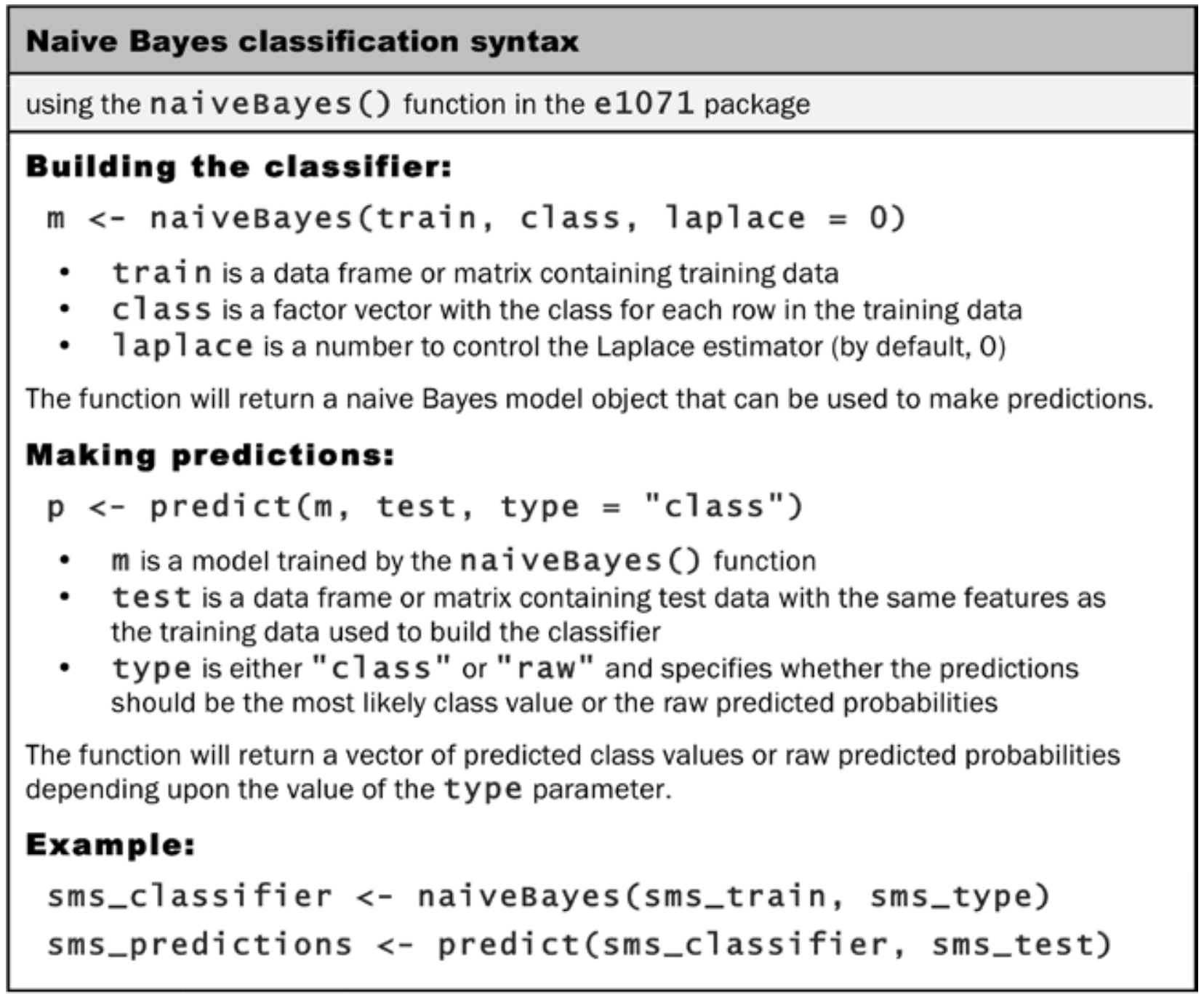
sms_classifier_1 <- naiveBayes(sms_train, sms_raw_train$type)
sms_test_pred_1 <- predict(sms_classifier_1, sms_test)

#########################################
## Part 4. Evaluating model performance #
#########################################

install.packages("gmodels")
library(gmodels)

CrossTable(x = sms_raw_test$type, y = sms_test_pred_1, prop.chisq=FALSE)
mean(sms_test_pred_1==sms_raw_test$type)


#########################################
## Part 5. Improving model performance #
#########################################

sms_classifier_2 <- naiveBayes(sms_train, sms_raw_train$type, laplace = 1)
sms_test_pred_2 <- predict(sms_classifier_2, sms_test)
CrossTable(x = sms_raw_test$type, y = sms_test_pred_2, prop.chisq = FALSE)
mean(sms_test_pred_2==sms_raw_test$type)

Linear Regression

lm() 是R语言中经常用到的函数,用来拟合回归模型。它是拟合线性模型最基本的函数。

1
myfit <- lm(formula,data)

其中,formula 指要拟合的模型形式,data 是一个数据框,包含了用于拟合模型的数据。

表达式(formula)形式如下:

1
Y~X1+X2..Xn

实例:

1
2
3
4
5
6
7
8
9
10
11
12
13
14
15
16
17
18
19
20
21
22
23
24
25
26
27
28
29
30
31
32
33
34
35
36
37
38
39
40
41
42
43
44
45
46
47
48
49
50
51
52
53
54
55
56
57
58
59
60
61
62
63
64
65
66
67
68
69
70
71
72
73
74
75
76
77
78
79
80
81
82
83
84
85
86
87
88
89
90
91
92
93
94
95
96
97
98
99
100
101
102
103
104
105
106
107
108
109
110
111
112
113
114
115
116
117
118
119
120
121
122
123
124
125
126
127
128
129
130
131
132
133
134
135
136
137
138
139
140
141
142
143
144
145
146
147
148
149
150
151
152
153
154
155
156
157
158
159
160
161
162
163
164
165
166
167
168
###########################################################
# Example. Linear Regression with Boston Housing Data #
###########################################################


###############
## Load Data ##
###############
library(MASS)
data(Boston)
colnames(Boston)

######################
## Data Exploration ##
######################

dim(Boston)
names(Boston)
str(Boston)
summary(Boston)

######################
## Data Preparation ##
######################

## Splitting data to training and testing samples
## we sample 90% of the original data and use it as the training set

sample_index <- sample(nrow(Boston),nrow(Boston)*0.90)
Boston_train <- Boston[sample_index,]
Boston_test <- Boston[-sample_index,]

## (Optional) Standardization

Boston$sd.crim <- (Boston$crim-mean(Boston$crim))/sd(Boston$crim);

Boston$sd.crim <- scale(Boston$crim);

for (i in 1:(ncol(Boston_train)-1)){
Boston_train[,i] <- scale(Boston_train[,i])
}


#####################
## Model Building ##
#####################

model_1 <- lm(medv~crim+zn+chas+nox+rm+dis+rad+tax+ptratio+black+lstat, data=Boston_train)
model_1 <- lm(medv~., data=Boston_train)
summary(model_1)

## Interaction terms in model
lm(medv~crim+zn+crim:zn, data=Boston_train)
#The following way automatically add the main effects of crim and zn
lm(medv~crim*zn, data=Boston_train)

#######################
## Model Assessment ##
#######################

## In-sample model evaluation (train error)

model_summary <- summary(model_1)
(model_summary$sigma)^2
## R2 of the model
model_summary$r.squared
model_summary$adj.r.squared
AIC(model_1)
BIC(model_1)


## Out-of-sample prediction (test error)

#pi is a vector that contains predicted values for test set.
pi <- predict(object = model_1, newdata = Boston_test)
## Mean Square Error
mean((pi - Boston_test$medv)^2)
## Mean Absolute Error (MAE)
mean(abs(pi - Boston_test$medv))
## Note that if you ignore the second argument of predict(), it gives you the in-sample ## prediction on the training set:

predict(model_1)
## Which is the same as
model_1$fitted.values


########################
## Variable Selection ##
########################

## Compare Model Fit Manually
model_1 <- lm(medv~., data = Boston_train)
model_2 <- lm(medv~crim+zn, data = Boston_train)
summary(model_1)
summary(model_2)
AIC(model_1); BIC(model_1)
AIC(model_2); BIC(model_2)


## Best Subset Regression
## The ‘leaps’ package provides procedures for best subset regression.

install.packages('leaps')
library(leaps)
#regsubsets only takes data frame as input
subset_result <- regsubsets(medv~.,data=Boston_train, nbest=2, nvmax = 14)
summary(subset_result)
names(summary(subset_result))
coef(subset_result,1:25)
coef(subset_result,21)
vcov(subset_result,21)
summary(subset_result)$which
summary(subset_result)$outmat
summary(subset_result)$bic

summary(subset_result)$which[which(summary(subset_result)$bic==min(summary(subset_result)$bic)),]

plot(subset_result, scale="bic")


#####################################################
## Best Subset Regression with package "lmSubsets" ##
#####################################################

install.packages("lmSubsets")
library(lmSubsets)

boston_select <- lmSelect(medv~.,data=Boston_train, penalty = "BIC", nbest = 1)
boston_best<-refit(boston_select)
summary(boston_best)
pred <- predict(boston_best, newdata=Boston_test)
SSE <- sum((pred-Boston_test$medv)^2)
SST <- sum((Boston_test$medv-mean(Boston_test$medv))^2)
1-SSE/SST


## Forward/Backward/Stepwise Regression Using AIC
## To perform the Forward/Backward/Stepwise Regression in R, we need to define the starting ## points:

nullmodel=lm(medv~1, data=Boston_train)
fullmodel=lm(medv~., data=Boston_train)
## nullmodel is the model with no varaible in it, while fullmodel is the model with every variable in it.

##########################
## Backward Elimination ##
##########################
model_step_b <- step(fullmodel,direction='backward')

########################
## Forward Selection ##
########################
model_step_f <- step(nullmodel, scope=list(lower=nullmodel, upper=fullmodel), direction='forward')

########################
## Stepwise Selection ##
########################
model_step_s <- step(nullmodel, scope=list(lower=nullmodel, upper=fullmodel), direction='both')
summary(model_step_s)
extractAIC(model_step_s)
extractAIC(model_step_s)[2]


## use a smaller set of variables
model_step_s <- step(nullmodel, scope=~lstat + rm + ptratio + dis + nox + chas + black + zn + crim, direction='both')

summary(model_step_s)
extractAIC(model_step_s)[2]

Logistic Regression

1
2
3
4
5
6
7
8
9
10
11
12
13
14
15
16
17
18
19
20
21
22
23
24
25
26
27
28
29
30
31
32
33

###########################################################
# Example 2. Logistic Regression with Lending Club Data #
###########################################################


# loans = read.csv("loans_full.csv")
# loans2 = loans[,c("not.fully.paid", "installment", "log.annual.inc", "fico", "revol.bal", "inq.last.6mths", "pub.rec")]
# write.csv(loans2, "loans.csv", row.names=F)

loans2 <- read.csv("loans.csv")
library(caret)
idx = createDataPartition(loans2$not.fully.paid, p = 0.7, list = FALSE)
train <- loans2[idx,]
test <- loans2[-idx,]

table(train$not.fully.paid)

## Estimate Logistic Regression Model
mod <- glm(not.fully.paid~., data=train, family="binomial")

## Predict Probabilities
pred <- predict(mod, newdata=test, type="response")
pred[1:10]
hist(pred)

## Tranform Probabilities into Classes
pred_class <- ifelse(pred>=0.2, 1, 0)


## Evaluate Test Data Prediction Performance
CrossTable(x = test$not.fully.paid, y = pred_class, prop.chisq=FALSE)
mean(test$not.fully.paid == pred_class)

Random Forest

1
2
3
4
5
6
7
8
9
10
library(randomForest)

RF.train=randomForest(Default~.,train_n)
print(RF.train)
importance(RF.train)

RF.pred=predict(RF.train,test_n,type="class")

pred_class4 <- ifelse(RF.pred>=0.5, 1, 0)
mean(test_n$Default == pred_class4)